3西格玛计算matlab,使用Matlab计算Efficient frontier

寻找slope最大点的函数

function [ port, opt_mu, opt_sigma ] = highest_slope_portfolio( R, RF, mu, sigma )

% This function finds the portfolio with the largest slope

% this function can easily be much more general

% e.g. mu, RF, sigma can be parameters

if nargin

return

elseif nargin == 1

RF=0.02;

mu=[.1 .2]’;

sigma=[.1 .2]’;

elseif nargin == 2

mu=[.1 .2]’;

sigma=[.1 .2]’;

end

% Here we use our define correlation coefficient

C=diag(sigma)*R*diag(sigma);

A=2*C;

A(:,end+1)=-(mu-RF);

A(end+1,1:end-1)=(mu-RF)’;

Rp=mu(1);

b=zeros(length(mu),1);

b(end+1,1)=Rp-RF;

x=inv(A)*b;

xopt=x(1:length(mu))./sum(x(1:length(mu)))’;

% Return value

port = xopt;

opt_mu = xopt’ * mu;

opt_sigma = sqrt( xopt’ * C * xopt);

end

案例 对比有无 无风险借贷的lending 和 borrowing:

Find the efficient frontier where short sales are allowed with and without risk less lending and borrowing. The following is given and does not change through question one of the assignment.

The risk free rate Rf is 2 %

Asset 1 yearly expected return is 10% and the standard deviation is 10%

Asset 2 yearly expected return is 20% and the standard deviation is 20%

For each of the following correlation coefficient between assets 1 and 2: rho=1; rho=0.5; rho=0; rho=-1

For Pepsi, Coca-Cola and Microsoft, estimate the yearly return, and covariance matrix of assets returns.

% To prevent unnessary loading of data from yahoo finance we add the if

% statement

if ~exist(‘stocks’, ‘var’)

stocks=hist_stock_data(‘01011991′,’01012001′,’PEP’, ‘KO’,’MSFT’,’frequency’,’wk’);

Pepsi = stocks(1);

CocaCola = stocks(2);

Microsoft = stocks(3);

end

% Caclualte log returns

PEPLR = log(Pepsi.AdjClose(2:end)./Pepsi.AdjClose(1:end-1) );

CCLR = log(CocaCola.AdjClose(2:end)./CocaCola.AdjClose(1:end-1) );

MSLR = log(Microsoft.AdjClose(2:end)./Microsoft.AdjClose(1:end-1) );

LogReturns = [ PEPLR, CCLR, MSLR ];

ymean = 52 * mean(LogReturns)’;

ystd = sqrt (52 * var(LogReturns))’;

ycorr = corr(LogReturns)’; %mistake was cor before

Calculate the efficient frontier with and without risk less lending and borrowing.

% These is constant throughout the excercise

RF = .02;

xopt = cell(2);

% Calculate the highest slope protfolio with each

[xopt{1}, muopt(1), sigopt(1)] = highest_slope_portfolio( ycorr(1:2, 1:2), RF, ymean(1:2), ystd(1:2) );

[xopt{2}, muopt(2), sigopt(2)] = highest_slope_portfolio( ycorr, RF, ymean, ystd);

% Plotting point by point

hold on;

plot (sigopt(1), muopt(1) , ‘x’);

hold on;

plot (sigopt(2), muopt(2) , ‘go’);

% As we know RF = 2% we can already plot the differnet efficient frontiers

% The starting point is always the same. 0 risk 2%

hold on;

plot (0, .02, ‘o’);

hold on;

RF_p1 = [0 sigopt(1) 2* sigopt(1)];

opt1_p = [.02 muopt(1) (2 * muopt(1) – RF) ];

line(RF_p1, opt1_p );

hold on;

RF_p2 = [0 sigopt(2) 2* sigopt(2)];

opt2_p = [.02 muopt(2) (muopt(2) * 2 – RF)];

line(RF_p2, opt2_p, ‘Color’,[1 0 0]);

% We can find ANOTHER efficient portfolio on the frontier, by running the

% same optimization with a DIFFERENT interscept

% Calculate the highest slope protfolio with each

xopt2 = cell(2);

[xopt2{1}, muopt2(1), sigopt2(1)] = highest_slope_portfolio( ycorr(1:2, 1:2), .05, ymean(1:2), ystd(1:2) );

[xopt2{2}, muopt2(2), sigopt2(2)] = highest_slope_portfolio( ycorr, .05, ymean, ystd);

%[xopt2(3,:), muopt2(3), sigopt2(3)] = highest_slope_portfolio( R{3}, .05);

%[xopt2(4,:), muopt2(4), sigopt2(4)] = highest_slope_portfolio( R{4}, .05);

% This is what we do, look for optimal point if the RF rate was 5%

% I Plot this too to show the idea

hold on;

plot (0, .05, ‘o’);

% Plotting the 2nd point on the portfolio

hold on;

plot (sigopt2(1), muopt2(1) , ‘go’);

hold on;

plot (sigopt2(2), muopt2(2) , ‘co’);

C = cell(2,1);

% Define the corresponding correlation matrices

C{1}=diag(ystd(1:2))*ycorr(1:2,1:2)*diag(ystd(1:2));

C{2}=diag(ystd)*ycorr*diag(ystd);

% As seen in class we have a general formula for finding the mean variance

% portfolio for two assets –

large_n = 100;

k = 20;

mu_p = zeros(4, 4*k* large_n + 1);

std_p = zeros(4, 4*k* large_n + 1);

%SR

% We will go through different combinations to find the efficient frontier;

for j = 1:2

for i = -2*k* large_n:1:2 * 2*k*large_n

curr_port = i / large_n * xopt2{j} + (1 – i / large_n) * xopt{j};

mu_p (j, i + 2*k * large_n + 1) = curr_port’ * ymean(1:j+1);

std_p(j, i + 2*k * large_n + 1) = sqrt(curr_port’ * C{j} * curr_port);

end

end

% SR =( mu_p – RF) ./ std_p

%find (max(SR) == SR)

%Plotting the efficient frontiers

hold on;

plot( std_p(1,:), mu_p(1,:));

%pause;

hold on;

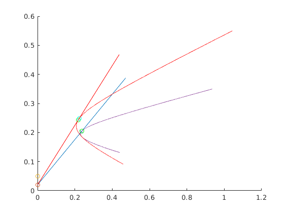
plot( std_p(2,:), mu_p(2,:), ‘r’);

得到的图案:

原文出处：https://www.cnblogs.com/hanani/p/10094544.html

相关资源：SRTApp:学生投票追踪器-其它代码类资源-CSDN文库